

First let's see how we can perform a single simulation, then we will see how to perform multiple simulations and visualize the Weak Law of Large Numbers.
Single Simulation 
Say that you want to know the average height of your classroom students. There are
\(300\)
students and you want to know, what is the average height of those \(300\)
students?You can't measure height of all
\(300\)
students, so you took small sample of \(50\)
students and measure their heights. Suppose that the average height of those \(50\)
students (sample mean) is somewhat near to the average height of all \(300\)
students (true mean). So the population size
\((N)\)
is \(300\)
and sample size\((n)\)
is \(50\)
. Remember that dogma
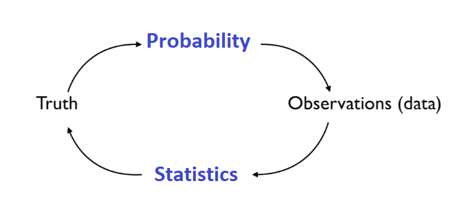
Truth
Now let's define the truth.Say that the each student's height follows the Normal distribution with mean
\((\mu)= 175 \text{cm}\)
and variance \((\sigma^2)=(10\text{cm})^2\)
. So
\(X_1,\cdots,X_{50}\sim\mathcal{N}(175,10^2)\)
Here we can argue that Normal distribution take values between\((-\infty,\infty)\), but heights aren't negative.
Clarification:
Yes\(\mathcal{N}(175,10^2)\)can take negative values but for\(\mathcal{N}(175,10^2)\)probability of taking negative values in insanely small.
Probability
Here we apply probability to generate data using the Truth we defined above.Now let's create the population of all
\(300\)
students. using Plots, Distributions, Random, Statistics
μ, σ = 175, 10
N = 300 # population size
""" 𝐗 ∼ 𝑵(μ, σ); mean = μ, variance = σ² """
# For clarification:
# Our notation of Normal distribution is N(mean, variance)
# And Julia's notation is N(mean, standard_deviation)
distribution = Normal(μ, σ)
""" "population" is vector of observation X₍₁₎, X₍₂₎, ..., X₍ₙ₎ """
population = rand(distribution, N)
Observation
Now that we have all\(300\)
students, and every student's height follows the Normal distribution with mean \((\mu)= 175 \text{cm}\)
and variance \((\sigma^2)=(10\text{cm})^2\)
. Let's (randomly) take a sample of
\(50\)
students. n = 50
sample_ = sample(population,n)
Statistics
So now that we have our sample of\(50\)
students, let's estimate the average height of those \(50\)
students (sample mean). sample_mean = mean(sample_)
But wait this is not the Weak Law of Large Numbers, it's just a sample mean.
Exactly this is not the Weak Law of Large Numbers, but to visualize the Weak Law of Large Numbers we just need to perform this simulation with increasing sample size
\((n)\)
and see if our sample mean converges to \(175\text{cm}\)
. So let's dive into it.
Multiple simulations
The truth is that every student's height follows the Normal distribution with mean \((\mu)= 175 \text{cm}\)
and variance \((\sigma^2)=(10\text{cm})^2\)
. First create a population
using Plots, Distributions, Random, Statistics
gr(fmt = :png, size = (1540, 810))
Random.seed!(1)

μ, σ = 175, 10
N = 300  # population size
"""  𝐗 ∼ 𝑵(μ, σ); mean = μ, variance = σ²  """
# For clarification:
# Our notation of Normal distribution is N(mean, variance)
# And Julia's notation is N(mean, standard_deviation)
distribution = Normal(μ, σ)

population = rand(distribution, N)
Now take sample mean for
\(n=1\)
to \(n=300\)
then plot them and observe the trend. Do the sample mean converges as sample size \((n)\)
increases? x_axis = 1:N # [1,2,...,N]
""" "sample_mean" is vector of running average ̅X₍₁₎, ̅X₍₂₎, ..., ̅X₍ₙ₎ """
sample_mean = cumsum(population) ./ (x_axis)
title = nameof(typeof(distribution))
""" plot vertical line for every observation; X₍₁₎, X₍₂₎, ⋯ X₍ₙ₎"""
plot(repeat((x_axis)', 2), [zeros(1, N) .+ μ; (population)'], label = "", color = :grey, alpha = 0.4)
""" plot observation; X₍₁₎, X₍₂₎, ⋯ X₍ₙ₎"""
plot!(x_axis, population, color = :grey, markershape = :circle, alpha = 0.5, label = "", linewidth = 0)
""" plot dashed line y=μ """
hline!([μ], color = :black, linewidth = 1.5, linestyle = :dash, grid = false, label = "")
plot!(x_axis, sample_mean, linewidth = 3, alpha = 0.6, color = :green, label = "| ̅Xₙ |")
xlabel!("n")
ylabel!("| ̅Xₙ |")
plot!(title = title)
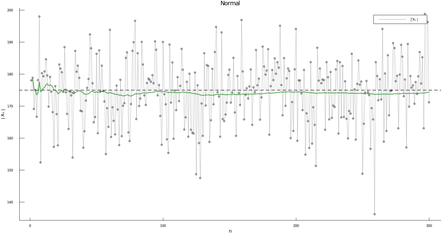
x-axis represents number of students
y-axis represents random variable
Here in this simulation we can see that as \((n)\)
y-axis represents random variable
\(\overline{X}_n\)
\(n\)
increases \(\overline{X}_n\)
do approaches to \(\mu\)
. Try playing with parameters, also try different distributions.
Simulation
Visualize Weak Law of Large Numbers
Try different distributions, tweak there parameters, and see how it impacts the convergence of\(\overline{X}_n\).