
The Counting Balls (Example) 
Say we have a room full of Red balls and Blue balls. We want to determine proportion of Red balls and Blue balls in that room, But we won't be able to count all the balls in the room as there are too many of them.
So we took a small sample of balls from that room to find the proportion of Red balls and Blue balls in that sample and hope that proportion we just estimated is somewhat near the True proportion(for the whole room).
Remember that dogma we showed previously.
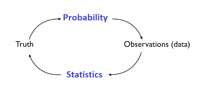
Truth
Let's first define the underlying truth, say that currently the room is holding\(40\%\)
of Red balls and \(60\%\)
of Blue balls. Note that we do not know this proportion and our intent is to find this proportion.Say we denote Red balls by "
\(1\)
" and Blue balls by "\(0\)
". Probability
We use probability to generate our data using the Truth we defined above.Now let's create a Population, in following scenario i.e. "All the balls in the room" .
(In this example we are creating
\(5000\)
balls and \(40\%\)
of them are Red balls ). # First of all import the libraries
import numpy as np
import matplotlib.pyplot as plt
N = 5000
true_proportion_for_red = 0.40
population = np.zeros(shape=N, dtype=int)
population[0:int(true_proportion_for_red*N)] = 1
np.random.shuffle(population)
\(40\%\)
of Red balls and \(60\%\)
of Blue balls. Observation
As we can see the room is full of\(5000\)
balls, and we can't count all of them to find out the proportion of Red balls and Blue balls. So we will take a sample(\(n\)
) out of those \(5000\)
balls to find the proportion of Red balls and Blue balls in that small sample. n=300
sample = np.random.choice(population,n)
\(300\)
balls. These
\(300\)
observations (\(X_1,\cdots,X_{300}\)
) are what we call Random Variables. Statistics
So now we have our sample of\(300\)
balls, let's start finding an estimate for Red balls proportion and Blue balls proportion. To find the proportion of Red balls, we count number of Red balls then we divide it by total number of balls (i.e.
\(300\)
). \(\hat{p}\)
: Our estimate for proportion of Red balls denoted by \(1\)
. \(\hat{q}\)
: Our estimate for proportion of Blue balls denoted by \(0\)
. \[ \hat{p} = \frac{1}{300}\sum_{i=0}^{300}X_i\]
\[ \hat{q} = 1-\hat{p} \]
p_hat = sum(sample)/n
q_hat = 1- p_hat
\(\hat{p}\)
).This is a single simulation, if we perform this simulation multiple times we can get some insights for the distribution of our Random variable
\(\hat{p}\)
. Multiple simulations
import numpy as np
import matplotlib.pyplot as plt
np.random.seed(1)

n_simulations = 1000	# Number of simulations
N = 5000				# population size
n = 300				 # sample size
p = 0.40				# True proportion of red balls
estimators = []		 # Here we store estimates of every simulation

# population: all 5000 balls
population = np.zeros(shape=N, dtype=int)
population[0:int(p*N)] = 1
np.random.shuffle(population)

for _ in range(n_simulations):
	# extract sample from population
	sample = np.random.choice(population,n)
	estimators.append(sum(sample)/n)
plt.xlabel("Proportion of Red balls")
plt.ylabel("Counts")
plt.hist(estimators, rwidth=0.95, bins=18)
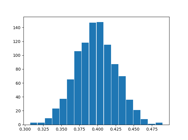
Does this (bell) curve seems familiar?
Simulation
Launch Statistics App