Gaussian Distribution

Gaussian Distribution (a.k.a. Normal distribution, Bell curve) is perhaps the most important probability distribution in statistics. We can see it in numerous natural phenomena like: heights, weight, age, measurement error, IQ score, etc.
We had already witnessed it's importance in Central Limit Theorem.

Gaussian Distribution

Notation	$\mathcal{N}(\mu,\sigma^2)$	Here $\mu$ and $\sigma^2$ are parameters Where $-\infty < \mu < +\infty$ And $\sigma^2 \gt \infty$
PDF	$f(x)=\frac{1}{\sigma \sqrt{2\pi }} \exp \left(-\frac{(x-\mu )^2}{2 \sigma ^2}\right)$	$-\infty \lt x \lt \infty$
CDF	$F(x)=\frac{1}{\sigma \sqrt{2\pi }} \int_{-\infty}^{x}\exp \left(-\frac{(t-\mu )^2}{2 \sigma ^2}\right)dt$	There is no closed form solution, for CDF of a Normal distribution

Notation	$\mathcal{N}(\mu,\sigma^2)$ Here $\mu$ and $\sigma^2$ are parameters Where $-\infty < \mu < +\infty$ And $\sigma^2 \gt \infty$
PDF	$f(x)=\frac{1}{\sigma \sqrt{2\pi }} \exp \left(-\frac{(x-\mu )^2}{2 \sigma ^2}\right)$ $-\infty \lt x \lt \infty$
CDF	$F(x)=\frac{1}{\sigma \sqrt{2\pi }} \int_{-\infty}^{x}\exp \left(-\frac{(t-\mu )^2}{2 \sigma ^2}\right)dt$ There is no closed form solution, for CDF of a Normal distribution

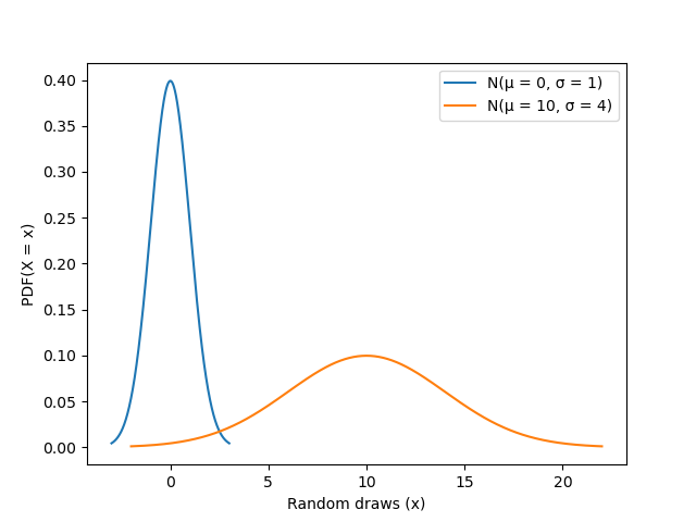
Python code to plot this distribution

import numpy as np
import matplotlib.pyplot as plt
def gaussian_plot(mu: float,
                  sigma: float,
                  partitions: int = 1000):
    rvs = np.linspace(mu - 3 * sigma, mu + 3 * sigma, partitions)
    pdf = (1/(sigma*np.sqrt(2*np.pi))) * np.exp(-((rvs-mu)**2)/(2*sigma**2))
    plt.plot(rvs, pdf, label = f"N(μ = {mu}, σ = {sigma})")
    plt.legend()
    plt.show()

gaussian_plot(0,1)
gaussian_plot(10,4)

Properties of Gaussian

The Empirical Rule

(\text{a.k.a. }68-95-99.7\text{ rule})

says: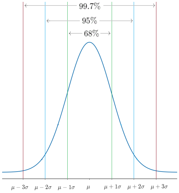

$68\%$ of population lies within $$1$$ standard deviation $(\sigma)$ from the mean $(\mu)$ .
$95\%$ of population lies within $$2$$ standard deviation $(\sigma)$ from the mean $(\mu)$ .
$99.7\%$ of population lies within $$3$$ standard deviation $(\sigma)$ from the mean $(\mu)$ .

Linear functions of Normal random variable

Gaussians are invariant under affine(linear) transformation, it means when we do a linear transformation of a Gaussian random variable, it remains a Gaussian random variable.
Like if

X\sim\mathcal{N}(\mu,\sigma^2)

and

\(Y=aX+b\)

then

Y\sim\mathcal{N}(a\mu+b,a^2\sigma^2)

Explanation

Standardization (a.k.a. Normalization/Z-score)

As we know that CDF of Gaussian distribution has no close form, so we can't solve it by hand. So we need a computer to do it for us. But the problem is, there are so many Gaussian r.v. with different

\mu

and

\sigma^2

.
The solution for this is Standardization. By it we can convert any Gaussian r.v. to a Standard Gaussian r.v

\mathcal{N}(0,1)

.
If

X\sim\mathcal{N}(\mu,\sigma^2)

then:

X-\mu\sim\mathcal{N}(0,\sigma^2)

\frac{X-\mu}{\sigma}\sim\mathcal{N}(0,1)

\Rightarrow Z=\frac{X-\mu}{\sigma}\sim\mathcal{N}(0,1)

Now we can compute probabilities for any Gaussian distribution:

\mathbb{P}\left(u\lt X\lt v\right)=\mathbb{P}\left(\frac{u-\mu}{\sigma} \lt Z \lt \frac{v-\mu}{\sigma}\right)

Symmetry

Any Gaussian r.v. with mean

(\mu)=0

is symmetric
If

X\sim \mathcal{N}(0,\sigma^2)

then

\(-X\)

has the same distribution as

\(X\)

\Rightarrow -X \sim \mathcal{N}(0,\sigma^2)

Gaussian Probability Table

So as we know that CDF of a gaussian has no close form, therefore we use tables to get those CDF's.
The table given below gives us CDF of a Standard Gaussian r.v.

\mathcal{N}(0,1)

CDF of

\mathcal{N}(0,1)=\Phi(x)

\Phi(x)=\mathbb{P}(\mathcal{N}(0,1) \leq x)=\frac{1}{\sqrt{2\pi }} \int_{-\infty}^{x}\exp \left(-\frac{t^2}{2}\right)dt

\text{Table for }\Phi(x)

z	+0.00	+0.01	+0.02	+0.03	+0.04	+0.05	+0.06	+0.07	+0.08	+0.09
0.0	0.50000	0.50399	0.50798	0.51197	0.51595	0.51994	0.52392	0.52790	0.53188	0.53586
0.1	0.53983	0.54380	0.54776	0.55172	0.55567	0.55966	0.56360	0.56749	0.57142	0.57535
0.2	0.57926	0.58317	0.58706	0.59095	0.59483	0.59871	0.60257	0.60642	0.61026	0.61409
0.3	0.61791	0.62172	0.62552	0.62930	0.63307	0.63683	0.64058	0.64431	0.64803	0.65173
0.4	0.65542	0.65910	0.66276	0.66640	0.67003	0.67364	0.67724	0.68082	0.68439	0.68793
0.5	0.69146	0.69497	0.69847	0.70194	0.70540	0.70884	0.71226	0.71566	0.71904	0.72240
0.6	0.72575	0.72907	0.73237	0.73565	0.73891	0.74215	0.74537	0.74857	0.75175	0.75490
0.7	0.75804	0.76115	0.76424	0.76730	0.77035	0.77337	0.77637	0.77935	0.78230	0.78524
0.8	0.78814	0.79103	0.79389	0.79673	0.79955	0.80234	0.80511	0.80785	0.81057	0.81327
0.9	0.81594	0.81859	0.82121	0.82381	0.82639	0.82894	0.83147	0.83398	0.83646	0.83891
1.0	0.84134	0.84375	0.84614	0.84849	0.85083	0.85314	0.85543	0.85769	0.85993	0.86214
1.1	0.86433	0.86650	0.86864	0.87076	0.87286	0.87493	0.87698	0.87900	0.88100	0.88298
1.2	0.88493	0.88686	0.88877	0.89065	0.89251	0.89435	0.89617	0.89796	0.89973	0.90147
1.3	0.90320	0.90490	0.90658	0.90824	0.90988	0.91149	0.91308	0.91466	0.91621	0.91774
1.4	0.91924	0.92073	0.92220	0.92364	0.92507	0.92647	0.92785	0.92922	0.93056	0.93189
1.5	0.93319	0.93448	0.93574	0.93699	0.93822	0.93943	0.94062	0.94179	0.94295	0.94408
1.6	0.94520	0.94630	0.94738	0.94845	0.94950	0.95053	0.95154	0.95254	0.95352	0.95449
1.7	0.95543	0.95637	0.95728	0.95818	0.95907	0.95994	0.96080	0.96164	0.96246	0.96327
1.8	0.96407	0.96485	0.96562	0.96638	0.96712	0.96784	0.96856	0.96926	0.96995	0.97062
1.9	0.97128	0.97193	0.97257	0.97320	0.97381	0.97441	0.97500	0.97558	0.97615	0.97670
2.0	0.97725	0.97778	0.97831	0.97882	0.97932	0.97982	0.98030	0.98077	0.98124	0.98169
2.1	0.98214	0.98257	0.98300	0.98341	0.98382	0.98422	0.98461	0.98500	0.98537	0.98574
2.2	0.98610	0.98645	0.98679	0.98713	0.98745	0.98778	0.98809	0.98840	0.98870	0.98899
2.3	0.98928	0.98956	0.98983	0.99010	0.99036	0.99061	0.99086	0.99111	0.99134	0.99158
2.4	0.99180	0.99202	0.99224	0.99245	0.99266	0.99286	0.99305	0.99324	0.99343	0.99361
2.5	0.99379	0.99396	0.99413	0.99430	0.99446	0.99461	0.99477	0.99492	0.99506	0.99520
2.6	0.99534	0.99547	0.99560	0.99573	0.99585	0.99598	0.99609	0.99621	0.99632	0.99643
2.7	0.99653	0.99664	0.99674	0.99683	0.99693	0.99702	0.99711	0.99720	0.99728	0.99736
2.8	0.99744	0.99752	0.99760	0.99767	0.99774	0.99781	0.99788	0.99795	0.99801	0.99807
2.9	0.99813	0.99819	0.99825	0.99831	0.99836	0.99841	0.99846	0.99851	0.99856	0.99861
3.0	0.99865	0.99869	0.99874	0.99878	0.99882	0.99886	0.99889	0.99893	0.99896	0.99900
3.1	0.99903	0.99906	0.99910	0.99913	0.99916	0.99918	0.99921	0.99924	0.99926	0.99929
3.2	0.99931	0.99934	0.99936	0.99938	0.99940	0.99942	0.99944	0.99946	0.99948	0.99950
3.3	0.99952	0.99953	0.99955	0.99957	0.99958	0.99960	0.99961	0.99962	0.99964	0.99965
3.4	0.99966	0.99968	0.99969	0.99970	0.99971	0.99972	0.99973	0.99974	0.99975	0.99976
3.5	0.99977	0.99978	0.99978	0.99979	0.99980	0.99981	0.99981	0.99982	0.99983	0.99983
3.6	0.99984	0.99985	0.99985	0.99986	0.99986	0.99987	0.99987	0.99988	0.99988	0.99989
3.7	0.99989	0.99990	0.99990	0.99990	0.99991	0.99991	0.99992	0.99992	0.99992	0.99992
3.8	0.99993	0.99993	0.99993	0.99994	0.99994	0.99994	0.99994	0.99995	0.99995	0.99995
3.9	0.99995	0.99995	0.99996	0.99996	0.99996	0.99996	0.99996	0.99996	0.99997	0.99997
4.0	0.99997	0.99997	0.99997	0.99997	0.99997	0.99997	0.99998	0.99998	0.99998	0.99998

Source: https://en.wikipedia.org/wiki/Standard_normal_table#Cumulative

How to read the table:
The first 2 digits represent a row and 3rd digit represents a column.

Examples

Say that we want to calculate $\Phi(0.07)$
then first 2 digits " $$0.0$$ " of 0.07 gives us row number 1, and 3rd digit " $$7$$ " gives us column number 8, so $\Phi(0.07) = 0.52790$
z +0.00 +0.01 +0.02 +0.03 +0.04 +0.05 +0.06 +0.07 +0.08 +0.09
0.0 0.50000 0.50399 0.50798 0.51197 0.51595 0.51994 0.52392 0.52790 0.53188 0.53586
Now say that we want to calculate $\Phi(1.26)$
then first 2 digits " $$1.2$$ " of 1.26 gives us row number 17, and 3rd digit " $$6$$ " gives us column number 7, so $\Phi(1.26) = 0.89617$
z +0.00 +0.01 +0.02 +0.03 +0.04 +0.05 +0.06 +0.07 +0.08 +0.09
1.2 0.88493 0.88686 0.88877 0.89065 0.89251 0.89435 0.89617 0.89796 0.89973 0.90147
Now we can also find $\mathbb{P}( 0.07 \leq \mathcal{N}(0,1) \leq 1.26)$ :
See solution
$\mathbb{P}( 0.07 \leq \mathcal{N}(0,1) \leq 1.26)=$ $\mathbb{P}(\mathcal{N}(0,1) \leq 1.26)-\mathbb{P}(\mathcal{N}(0,1) \leq 0.07)$ $$=0.89617 - 0.5279=0.36827$$
Now let's calculate $\Phi(-0.07) = \mathbb{P}(\mathcal{N}(0,1) \leq -0.07)$
See solution
Say $Z=\mathcal{N}(0,1)$
$\mathbb{P}(Z \leq -0.07)=\mathbb{P}(-Z \geq 0.07)$
And $\mathbb{P}(-Z \geq 0.07)=\mathbb{P}(Z \geq 0.07)$ ;by symmetry
$\mathbb{P}(Z \geq 0.07)= 1- \mathbb{P}(Z \leq 0.07)$
$\mathbb{P}(Z \geq 0.07)= 1- \Phi(0.07)$
$\mathbb{P}(Z \geq 0.07)= 1- 0.52790=0.4721$
$\Rightarrow \Phi(-0.07)=0.4721$
Now let's calculate
$\mathbb{P}(|\mathcal{N}(0,1)| \gt 0.07)$
See solution
Say
$Z=\mathcal{N}(0,1)$

$\mathbb{P}(|Z| \gt 0.07)=\mathbb{P}(Z \gt 0.07 \cup Z \lt -0.07)=$

$ \mathbb{P}(Z \gt 0.07)+\mathbb{P}(Z\lt -0.07) $

And
- $\mathbb{P}(Z \gt 0.07) =1-\mathbb{P}(Z \leq 0.07)=$ $1-\Phi(0.07)=$ $$1 - 0.5279=0.4721$$
- $\mathbb{P}(Z\lt -0.07)=\Phi(-0.07)$ and we calculated above and $\Phi(-0.07)=0.4721$
So:
$\mathbb{P}(|Z| \gt 0.07)=0.4721+0.4721=0.9442$

And we can say that:
$\mathbb{P}(|Z| \gt x)= 2(1-\Phi(x)) $
Say
$ X\sim \mathcal{N}(70,36) $
now calculate
$\mathbb{P}(X>80)$
See solution
Say
$Z=\mathcal{N}(0,1)$

$ \mathbb{P}(X\gt 80) =\mathbb{P}(X-70 \gt 80-70)$

$\Rightarrow \mathbb{P}(X\gt 80) =\mathbb{P}(\frac{X-70}{6} \gt \frac{80-70}{6})$

$\Rightarrow \mathbb{P}(X\gt 80) =\mathbb{P}( Z \gt 1.66)$
- $\mathbb{P}(Z \gt 1.66)=1 - \mathbb{P}(Z \leq 1.66)$
  $\Rightarrow \mathbb{P}(Z \gt 3.33) = 1-0.95154 = 0.04846$
$\Rightarrow \mathbb{P}(X\gt 80) = 0.04846 $
Say
$X\sim \mathcal{N}(70,36)$
now we have to find
$x$
such that
$\mathbb{P}(X\leq x)=80\%$

Now we have to read the table backward.
See solution
Say
$Z=\mathcal{N}(0,1)$

$ \mathbb{P}(X\leq x) =0.8$

$\Rightarrow \mathbb{P}(X-70\leq x-70) =0.8$

$\Rightarrow \mathbb{P}\left(\frac{X-70}{6}\leq \frac{x-70}{6}\right) =0.8$

$\Rightarrow \mathbb{P}\left(Z \leq \frac{x-70}{6}\right) =0.8$

$\Rightarrow \Phi\left( \frac{x-70}{6}\right) =0.8$

z +0.00 +0.01 +0.02 +0.03 +0.04 +0.05 +0.06 +0.07 +0.08 +0.09
0.8 0.78814 0.79103 0.79389 0.79673 0.79955 0.80234 0.80511 0.80785 0.81057 0.81327
- $\Phi(0.85)=0.80$
$\Rightarrow \frac{x-70}{6}=0.85$

$\Rightarrow x=75.1$

z	+0.00	+0.01	+0.02	+0.03	+0.04	+0.05	+0.06	+0.07	+0.08	+0.09
1.2	0.88493	0.88686	0.88877	0.89065	0.89251	0.89435	0.89617	0.89796	0.89973	0.90147

z	+0.00	+0.01	+0.02	+0.03	+0.04	+0.05	+0.06	+0.07	+0.08	+0.09
0.8	0.78814	0.79103	0.79389	0.79673	0.79955	0.80234	0.80511	0.80785	0.81057	0.81327

Quantile

Here we have to find a number

q_\alpha

or say the quantile of order

1- \alpha

of a r.v.

\(X\)

such that the CDF of

\(X\)

q_\alpha

is:

F(q_\alpha)=\mathbb{P}(X \leq q_\alpha)=1-\alpha

Here we are just reading the table backward, So we are just computing

F^{-1}(x)

Some important quantiles of

Z\sim \mathcal{N}(0,1)

$\alpha$	$2.5\%$	$5\%$	$10\%$
$q_\alpha$	1.96	1.65	1.28

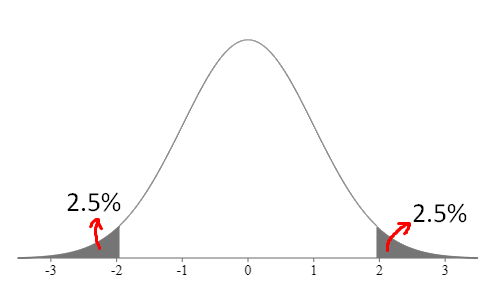
\mathbb{P}(|Z| \gt 1.96)=5\%

Now let's see an implementation, choose your language of choice,
,
Launch Statistics App

Gaussian Distribution