

First let's see how we can perform a single simulation, then we will see how to perform multiple simulations and visualize the Weak Law of Large Numbers.
Single Simulation 
Assume that there are \(1000\)
students in your school and you want to know, what is the average height of \(100\)
randomly selected students and how is that average height distributed (or say the distribution of that average height)?Remember that dogma
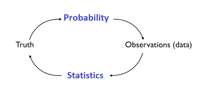
Truth
Now let's define the truth.Say that every student's height follows the Uniform distribution with range of
\([165\text{ cm },185\text{ cm}]\)
. So
\(X_1,\cdots,X_{50}\sim\text{Unif}[165, 185]\)
Note: This information is completely unknown to us.
Probability
Here we apply probability to generate data using the Truth we defined above.Now let's create the population of all
\(1000\)
students. import numpy as np
import matplotlib.pyplot as plt
from scipy.stats import uniform # to draw random variables from Uniform distribution
N = 1000 # population size
a = 165
scale = 20
# Unif[a, a + scale]
distribution = uniform(a, scale)
population = distribution.rvs(N)
Observation
Now that we have all\(1000\)
students, and every student's height follows the Uniform distribution. Let's (randomly) take a sample of
\(100\)
students. n = 100
sample = np.random.choice(population,n)
Statistics
So now we have our sample of\(100\)
students, let's estimate the average height of those \(100\)
students (sample mean). sample_mean = np.mean(sample)
\(100\)
randomly selected students. Now let's see how the distribution of the average height of
\(100\)
randomly selected students look like. To achieve this we need to perform this simulation multiple times and plot all sample means as a histogram.
Multiple simulations
The truth is that every student's height follows the Uniform distribution \(\text{Unif}[165, 185]\)
, so let's start with creating population. import numpy as np
import matplotlib.pyplot as plt
from scipy.stats import uniform # to draw random variables from Uniform distribution
np.random.seed(1)
N = 1000 # population size
a = 165
scale = 20
# Unif[a, a + scale]
distribution = uniform(a, scale)
population = distribution.rvs(N)
Now let's collect n_simulations sample means of sample size
\((n) = 30\)
. (say n_simulations = 200)
n = 30
n_simulations = 200
sample_means = np.zeros(n_simulations)
for k in range(n_simulations):
	sample_means[k] = np.mean(np.random.choice(population,n))
num_bins = 50
n, bins, patches = plt.hist(sample_means, num_bins, facecolor='blue', alpha=0.5)
plt.xlabel("Sample mean")
plt.ylabel("# occurrences of sample mean")
plt.show()
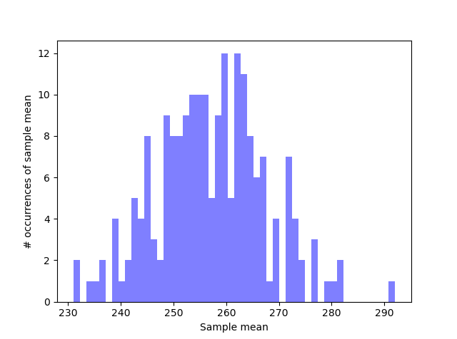
Sample mean seems to be normally distributed.
Well it's a Central Limit Theorem Simulation right, and the whole point of CLT is to approximate probability distribution of sample mean \(\overline{X}_n\)
to it's corresponding Normal distribution, am I correct? Let's see ourselves. Let's overlay a Normal distribution with true mean and variance of sample_means.
from scipy.stats import norm
samples_mean = np.mean(sample_means)
samples_std = np.std(sample_means)

fig, ax = plt.subplots()

# Getting PDF
x = np.linspace(samples_mean - 3*samples_std, samples_mean + 3*samples_std, 100)
pdf = norm.pdf(x, samples_mean, samples_std)
ax.plot(x, pdf, c="g", label="Normal distribution (PDF)")

# Getting Histogram
num_bins = 50
counts, bins = np.histogram(sample_means,
							np.linspace(min(sample_means),
										max(sample_means),
										num_bins)
							)
n, bins, patches = ax.hist(sample_means,
							bins[:-1],
							facecolor='blue',
							alpha=0.5,
							color="b",
							weights=(1/sum(counts))*np.ones_like(sample_means),
							label="Sampling distribution")
leg = ax.legend();
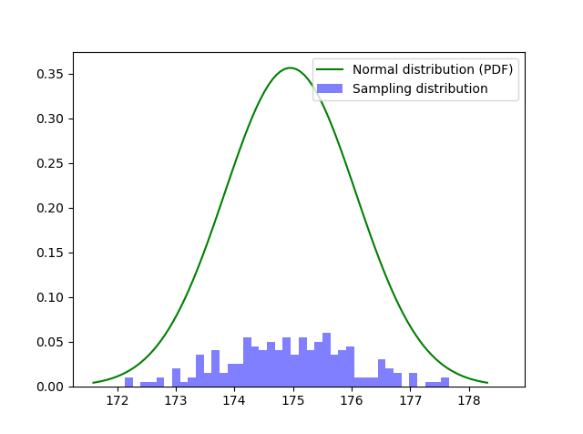 Here height of the bins of Sampling distribution represent the probability of falling into that bin.
 The Normal distribution that we plotted have same mean and variance as of our Sampling distribution, but their shapes are way off.
Sampling distribution of \(\sqrt{n}\, (\overline{X}_n-\mu)\) is much better fit for Normal distribution
If you follow the result of the CLT,\[\sqrt{n}\, (\overline{X}_n-\mu) \xrightarrow [n\to \infty ]{(d)} \mathcal{N}(0,\sigma^2) \]Then you can see our normally distributed data.
We just have to center our observations around\(0\)and then stretch it by a factor of\(\sqrt{n}\).from scipy.stats import norm mean = np.mean(np.sqrt(n) * (sample_means - distribution.mean())) std = np.sqrt(n) * np.std(sample_means) # Centered and stretched sample mean (r.v.) sample_means = np.sqrt(n) * (sample_means - distribution.mean()) fig, ax = plt.subplots() # Getting PDF N(0, σ) x = np.linspace(- 3*std, 3*std, 100) pdf = norm.pdf(x, 0, std) ax.plot(x, pdf, c="g", label="Normal distribution (PDF)") # Getting Histogram num_bins = 50 counts, bins = np.histogram(sample_means, np.linspace(min(sample_means), max(sample_means), num_bins) ) n, bins, patches = ax.hist(sample_means, bins[:-1], facecolor='blue', alpha=0.5, color="b", weights=(1/sum(counts))*np.ones_like(sample_means), label="Sampling distribution") leg = ax.legend();Now the plot feels much more Normal but here the random variable is
\(\sqrt{n}\, (\overline{X}_n-\mu) \)not\(\overline{X}_n\).
And as we discussed earlier that,
Central Limit Theorem is not a statement about the convergence of PDF or PMF. It's a statement about the convergence of CDF.Now let's see ourselves,
# Plot CDF
fig, ax = plt.subplots()
# CDF of Normal Distribution
cdf = norm.cdf(x, samples_mean, samples_std)
ax.plot(x, cdf, c='g', label="Normal distribution CDF")

# CDF of Sampling Distribution
cdf = np.cumsum(n)/sum(n)
ax.scatter(bins[:-1], cdf, c='b', marker="*", label="Sampling distribution CDF")
leg = ax.legend();
plt.show()
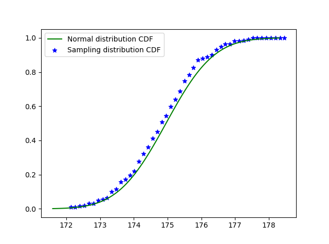 Here we can see the beauty of Central limit theorem, we can see how the CDF of our Sampling distribution get closer to the CDF of a Normal distribution.
 Now try tweaking
\(n\)
and see how it affects the CDF convergence. Also try different distributions form scipy.stats
Simulation
Visualize Central Limit Theorem
Try different distributions, tweak there parameters, sample size, number of simulations and see how it impacts the convergence of CDF of\(\overline{X}_n\).