Menu
QuantML.orgQuantML.org
  • Linear Algebra
  • Thanks

    Table of Content

    • \(1)\)
      Vector Space
       
      • \(1.0\)
             Introduction
      • \(1.1\)
             Vector Space Properties

    • \(2)\)
      Column Space
       
      • \(2.0\)
             Introduction
      • \(2.1\)
             Example in
        \(\mathbb{R}^3\)
      • \(2.2\)
             Example in
        \(\mathbb{R}^4\)
      • \(2.3\)
             Matrix Notation
      • \(2.4\)
             Dependency

    • \(3)\)
      Null Space
      \((A\vec{x}=\vec{0})\)
       
      • \(3.0\)
             Introduction
      • \(3.1\)
             Example in
        \(\mathbb{R}^4\)
      • \(3.2\)
             Is
        \(A\vec{x}=0\)
        a vector space?
      • \(3.3\)
          Elimination Technique
      • \(3.4\)
          pivot column/free columns
      • \(3.5\)
          Finding special solution
      • \(3.6\)
          # special solutions
      • \(3.7\)
          Reduced Row Echelon Form

    • \(4)\)
      Solving
      \(A\vec{x}=\vec{b}\)
       
      • \(4.0\)
             Introduction
      • \(4.1\)
             Find
        \(\vec{x}\)
        that solves
        \(A\vec{x}=\vec{b}\)
        ?
      • \(4.1.1\)
          Elimination Technique

    • \(5)\)
      Rank Of a Matrix
       
      • \(5.0\)
             Introduction
      • \(5.1\)
             Full column rank matrix
         
      • \(5.2\)
             Full row rank matrix
         
      • \(5.3\)
             Full rank matrix
         
      • \(5.4\)
             Dimensions and Basis
         
      • \(5.4.1\)
          Column Space
      • \(5.4.2\)
          Null Space

    • \(6)\)
      \(\mathbf{4}\)
      fundamental subspaces
       
      • \(6.0\)
             Introduction
      • \(6.1\)
             Row Space
         
      • \(6.2\)
             Left Null Space
         
        • \(6A)\)
               Dimensions of fundamental spaces
           
          • \(6A.1\)
                 Dimensions of Column space
          • \(6A.2\)
                 Dimensions of Null space
          • \(6A.3\)
                 Dimensions of Row space
          • \(6A.4\)
                 Dimensions of Left Null space
        • \(6B)\)
               Basis of fundamental spaces
           
          • \(6B.1\)
                 Basis of Column space
          • \(6B.2\)
                 Basis of Null space
          • \(6B.3\)
                 Basis of Row space
          • \(6B.4\)
                 Basis of Left Null space

    • \(7)\)
      Matrix Space
       
      • \(7.1\)
             Matrix
      • \(7.2\)
             Vector Interpretation
      • \(7.3\)
             Matrix Interpretation
      • \(7.4\)
             Vector interpretation of a Matrix
      • \(7.5\)
             Matrix space
      • \(7.5.1\)
          Lower Triangular
      • \(7.5.2\)
          Symmetric Matrix
        • \(7A)\)
          Dimensions and Basis
           
          • \(7A.1\)
                 Basis of all
            \(3\times 3\)
            matrices
          • \(7A.1.1\)
                 Lower Triangular
          • \(7A.1.1\)
                 Symmetric Matrix
        • \(7B)\)
          Operations on Subspaces
           
          • \(7B.1\)
                
            \(\mathcal{S} \cap \mathcal{U}\)
          • \(7B.2\)
                
            \(\mathcal{S} \cup \mathcal{U}\)
          • \(7B.3\)
                
            \(\mathcal{S} + \mathcal{U}\)
        • \(7C)\)
          More Examples
          • \(7C.1\)
                 More Examples on Matrix Space

    • \(8)\)
      Orthogonal Subspaces
       
      • \(8.0\)
             Introduction
      • \(8.1\)
             Orthogonal Vector
      • \(8.2\)
             Orthogonal Subspaces
      • \(8.3\)
             Row space is orthogonal to null space
      • \(8.4\)
             Column space is orthogonal to left null space

    • \(9)\)
      Projection
       
      • \(9.0\)
             Introduction
      • \(9.1\)
             Vector Projection
      • \(9.1.1\)
          Projection Matrix of a vector
      • \(9.2\)
             Why are we doing projection?
      • \(9.3\)
             Matrix Projection
      • \(9.3.1\)
          Projection onto the column space of a matrix
      • \(9.4\)
             Least Squares(Application of projection)

    • \(10)\)
      Orthonormal column Vectors
       
      • \(10.0\)
             Introduction
      • \(10.1\)
             What is the benefit of orthonormal column vector
      • \(10.2\)
             Gram Schmidt

    • \(11)\)
      Eigenvalues and Eigenvectors
       
      • \(11.0\)
             Introduction
      • \(11.1\)
             Solving
        \(A\vec{x}=\lambda\vec{x}\)

    • \(12)\)
      Diagonalization and Power of a Matrix
       
      • \(12.1\)
             Diagonalization of a Matrix
      • \(12.2\)
             Power of a matrix
      • \(12.3\)
             Fibonacci example

    • \(13)\)
      Differential Equation
       
      • \(13.1\)
             Matrix Exponential
      • \(13.2\)
             Differential Equation
      • \(13.3\)
             States

    • \(14)\)
      Markov Matrix & Fourier Series
       
      • \(14.0\)
             Introduction
      • \(14.1\)
             Example of Markov Matrices
      • \(14.2\)
             Expansion with Orthogonal basis
      • \(14.3\)
             Fourier Series

    • \(15)\)
      Symmetric Matrices Properties
       
      • \(15.0\)
             Introduction
      • \(15.1\)
             Properties

    • \(16)\)
      Complex Matrix & Fast Fourier Transform
       
      • \(16.1\)
             Complex Matrices
      • \(16.1.1\)
          Complex symmetric matrices
      • \(16.1.2\)
          Complex Orthonormal Vectors
      • \(16.2\)
             Fast Fourier Transform

    • \(17)\)
      Positive Definite Matrices
       
      • \(17.1\)
             Properties
      • \(17.2\)
             Examples

    • \(18)\)
      Similar Matrices
       
      • \(18.1\)
             Properties/Examples

    • \(19)\)
      Singular Value Decomposition
       
      • \(19.0\)
             Introduction
      • \(19.0.1\)
          Row Space
      • \(19.0.2\)
          Null Space
      • \(19.0.3\)
          Column Space
      • \(19.0.4\)
          Left Null Space
      • \(19.0.5\)
          Terminologies
      • \(19.1\)
             Full SVD
      • \(19.2\)
             Reduced SVD
      • \(19.3\)
             Finding
        \(V\)
        and
        \(U\)
        Orthonormal matrix
      • \(19.3.1\)
          Row space of
        \(A\)
        is same as Row space of
        \(A^TA\)
      • \(19.3.2\)
          Column Space of
        \(A\)
        is same as Column Space of
        \(AA^T\)
      • \(19.4\)
             Finding orthonormal Row vectors
        \((V)\)
        for matrix
        \(A\)
      • \(19.5\)
             Finding orthonormal Column Vectors
        \((U)\)
        for matrix
        \(A\)


    A space is a vector space if
    \(1)\)
      If there is a vector in the space and we multiply that vector with a constant
    \(c\in\mathbb{R}\)
    then the resulting vector must be in the space.
    \(2)\)
      Say we took two vectors
    \(\vec{v}\)
    and
    \(\vec{w}\)
    then there sum must be in that space.
    \(3)\)
      Vector space must pass through the origin.
    Say we have two vectors
    \(\vec{v}, \vec{w} \in \mathbb{R}^d\)
    .
    \(\bullet\)
      if
    \(\vec{v}\)
    is parallel to
    \(\vec{w}\)
    , then vector space of
    \(\vec{v}\)
    and
    \(\vec{w}\)
    is a space in
    \(\mathbb{R}\)
    (line)
    Column Space of a Matrix
    \(A \quad \left( C(A) \right)\)
    Say that shape of matrix
    \(A\)
    is
    \(m\times n\)
    ,
    \(A\in\mathbb{R}^{m\times n}\)
    .
    Column vector refers to column of a matrix.

    \(\bullet\)
      Linear Combination of these column vectors gives us the column space of matrix
    \(A\)
    .

    \(\bullet\)
      There maybe some dependent column vectors.
    \(\bullet\)
      Dependent column vectors can be achieved by the linear Combination of other column vectors.
    \(\bullet\)
      These dependent column vectors are redundant for our column space, if we remove these dependent column vectors from
    \(A\)
    our column space will be unaffected.
    Null Space of a Matrix
    \(A\)
    \( \quad \left( N(A) \right)\)
    Say that shape of matrix
    \(A\)
    is
    \(m\times n\)
    ,
    \(A\in\mathbb{R}^{m\times n}\)
    .
    \(\bullet\)
      For a matrix say
    \(A\)
    the Null space is the space of all
    \(\vec{x}\)
    that solves
    \(A\vec{x}=\vec{0}\)
    .

    \(\bullet\)
      Null space is a vectors space.
    There might be some dependent column vectors in matrix
    \(A\)
    , if there are some dependent column vectors then,
    \(\bullet\)
      If there are
    \(k\)
    dependent column vectors then our Null Space
    \(\in\mathbb{R}^k\)
    .
    \(\bullet\)
      If there is not any dependent column vectors then the Null Space is just the
    \(\vec{0}\)
    (zero vector), because
    \(\vec{x}=\vec{0}\)
    solves
    \(A\vec{x}=\vec{0}\)
    .
    \(\bullet\)
      Null Space of
    \(A\)
    is orthogonal to the Row Space of
    \(A\)
    .
    Solving
    \(A\vec{x}=\vec{b}\)
    Say that shape of matrix
    \(A\)
    is
    \(m\times n\)
    ,
    \(A\in\mathbb{R}^{m\times n}\)
    .
    \(A\vec{x}\)
    is just a linear combinations of column vector of matrix
    \(A\)
    , so the resultant of this linear combination must lie in the column space of
    \(A\)
    . So
    \(\bullet\)
     
    \(A\vec{x}=\vec{b}\)
    is solvable if
    \(\vec{b}\)
    lies in the column space of
    \(A\)
    .
    \(\bullet\)
      Complete solution of
    \(A\vec{x}=\vec{b}\)
    is
    \(\vec{x} = \vec{x}_p+\vec{x}_n\)

    \( \vec{x}_p\)
    is a particular solution for
    \(A\vec{x}=\vec{b}\)
    and,
    \(\vec{x}_n\)
    is the null space of matrix
    \(A\)
    .

    So any
    \(\vec{x}\in\vec{x}_p+\vec{x}_n\)
    solves
    \(A\vec{x}=\vec{b}\)

    Rank of a
    \(m\times n\)
    matrix
    \(A\)
    A rank is the number of pivots of matrix
    \(A\)
    .
    So we have
    \(n\)
    column vectors in
    \(\mathbb{R}^m\)
    , and there are
    \((n-r)\)
    (dependent)column vectors which we can get by the linear combination of other
    \(r\)
    (independent)column vectors.
    \(\bullet\)
      # pivots can't be
    \(\gt\)
    # rows (
    \(m\)
    ), so
    \(r\leq m\)

    \(\bullet\)
      # pivots can't be
    \(\gt\)
    # columns (
    \(n\)
    ), so
    \(r\leq n\)

    Full Column Rank of matrix
    \(A\)
    For a
    \(m\times n\)
    matrix
    \(A\)
    of rank
    \(r\)
    and
    \(m\gt n\)
    .
    \(\text{Rank}(A)=r=n\)
    it means that all of the column vectors are independent.
    \(\bullet\)
      # pivots
    \(=n\)
    \(\Rightarrow\)
    # dependent column vectors
    \(=0\)
    .
    Here we have no dependent column vectors here so,
    \(\bullet\)
      Null Space of
    \(A\)
    is just
    \(\vec{0}\)
    .
    So complete solution is just a single vector
    \(\vec{x}_p\)
    if it exists.
    # solution =
    \(\left\{\begin{matrix} 1 & \text{ if there is a solution} \\ 0 & \text{ otherwise} \\ \end{matrix}\right.\)

    Full Row Rank of matrix
    \(A\)
    For a
    \(m\times n\)
    matrix
    \(A\)
    of rank
    \(r\)
    and
    \(m\lt n\)
    .
    \(\text{Rank}(A)=r=m\)
    now all of the column vectors are not independent.
    \(\bullet\)
      # pivots
    \(=m\)
    \(\Rightarrow\)
    # dependent column vectors
    \(=n-r\)
    .
    Here we have
    \(n-r\)
    dependent column vectors so,
    \(\bullet\)
      Null Space of
    \(A\)
    is in
    \(\mathbb{R}^{n-r}\)
    .
    So complete solution have
    \(\infty\)
    possible solutions.
    \(\bullet\)
      # solutions are
    \(\infty\)

    Full Rank of matrix
    \(A\)
    For a
    \(m\times n\)
    matrix
    \(A\)
    of rank
    \(r\)
    and
    \(m = n\)
    .
    \(\text{Rank}(A)=r=n\)
    it means that all of the column vectors are independent.
    \(\bullet\)
      # pivots
    \(=n\)
    \(\Rightarrow\)
    # free column vectors
    \(=0\)
    .
    Here we have no dependent column vectors here so,
    \(\bullet\)
      Null Space of
    \(A\)
    is just
    \(\vec{0}\)
    .
    So complete solution is just a single vector
    \(\vec{x}_p\)
    and it is in the column space of our matrix
    \(A\)
    .
    \(\bullet\)
      # solutions
    \(=1\)

    Dimensions and Basis
    Say we have a matrix
    \(A_{m\times n}\in\mathbb{R}^{m\times n}\)

    Column Space
    \(\bullet\)
      Column Space of matrix
    \(A\)
    lives in
    \(\mathbb{R}^m\)
    .
    \(\bullet\)
      The basis for column space are (independent)pivot columns of matrix
    \(A\)
    .
    \(\bullet\)
      # Dimensions
    \(=\)
    # pivot columns
    \(=Rank(A)=r\)

    Null Space
    \(\bullet\)
      Null Space of matrix
    \(A\)
    also lives in
    \(\mathbb{R}^m\)
    .
    \(\bullet\)
      The basis for null space are special solutions of matrix
    \(A\)
    .
    \(\bullet\)
      # Dimensions
    \(=\)
    # special solutions
    \(=Rank(A)=r\)

    Row Space of a Matrix
    \(A\)
    \(\quad \left( C(A^T) \right)\)
    Say that shape of matrix
    \(A\)
    is
    \(m\times n\)
    ,
    \(A\in\mathbb{R}^{m\times n}\)
    .
    Row vectors refers to the rows of a matrix.
    \(\bullet\)
      Linear Combination of these row vectors gives us the row space of matrix
    \(A\)
    .

    \(\bullet\)
      There maybe some dependent row vectors.
    \(\bullet\)
      Dependent row vectors can be achieved by the linear Combination of other row vectors.
    \(\bullet\)
      These dependent row vectors are redundant for our row space, if we remove these dependent row vectors from
    \(A\)
    our row space will be unaffected.
    Left Null Space of a Matrix
    \(A\)
    \(\quad \left( N(A^T) \right)\)
    Say that shape of matrix
    \(A\)
    is
    \(m\times n\)
    ,
    \(A\in\mathbb{R}^{m\times n}\)
    .
    \(\bullet\)
      For a matrix say
    \(A\)
    the Left Null space is the space of all
    \(\vec{x}\)
    that solves
    \(A^T\vec{x}=\vec{0}\)
    .

    \(\bullet\)
      Left Null space is a vectors space.
    There might be some dependent row vectors in matrix
    \(A\)
    .
    \(\bullet\)
      If there are
    \(k\)
    dependent row vectors then our Left Null Space
    \(\in\mathbb{R}^k\)
    .
    \(\bullet\)
      If there is not any dependent row vectors then the Left Null Space is just the
    \(\vec{0}\)
    (zero vector), because
    \(\vec{x}=\vec{0}\)
    solves
    \(A^T\vec{x}=\vec{0}\)
    .
    \(\bullet\)
      Left Null Space of
    \(A\)
    is orthogonal to the Column Space of
    \(A\)
    .
    Fundamental Subspaces
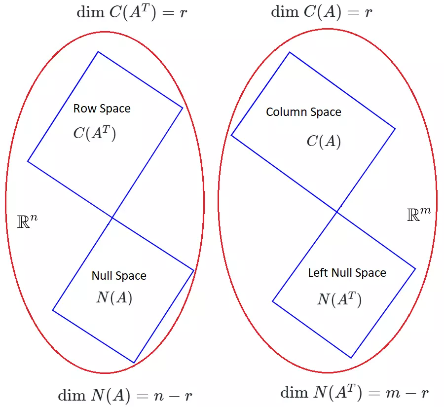
    There are
    \(4\)
    fundamental subspaces (say we have a
    \(m\times n\)
    matrix
    \(A\)
    ):
    \(1. \text{ Column Space } (C(A)) \)

    \(2. \text{ Null Space } (N(A)) \)

    \(3. \text{ Row Space } (C(A^T))\)

    \(4. \text{ Left Null Space } (N(A^T))\)

    Dimensions of fundamental spaces
    Say we have a
    \(m\times n\)
    matrix
    \(A\)
    ,
    \(A\in\mathbb{R}^{m\times n}\)
    and rank of matrix is
    \(r\)

    \(\bullet\)
      Column space lives in
    \(r\)
    dimensional vector space,
    \(C(A)\in\mathbb{R}^r\)

    \(\bullet\)
      Row space also lives in
    \(r\)
    dimensional vector space,
    \(C(A^T)\in\mathbb{R}^r\)

    \(\bullet\)
      Null space lives in
    \(n-r\)
    dimensional vector space,
    \(N(A)\in\mathbb{R}^{n-r}\)

    \(\bullet\)
      Left Null space lives in
    \(m-r\)
    dimensional vector space,
    \(N(A^T)\in\mathbb{R}^{m-r}\)

    Basis of fundamental spaces
    Say we have a
    \(m\times n\)
    matrix
    \(A\)
    ,
    \(A\in\mathbb{R}^{m\times n}\)
    and rank of matrix is
    \(r\)

    \(\bullet\)
      Basis of Column space are those
    \(r\)
    independent columns of matrix
    \(A\)

    \(\bullet\)
      Basis of Row space are those
    \(r\)
    independent rows of matrix
    \(A\)

    \(\bullet\)
      Basis of Null space are those
    \(n-r\)
    special solutions, which we can get by solving
    \(A\vec{x}=\vec{0}\)

    \(\bullet\)
      Basis of Left Null space are those
    \(m-r\)
    special solutions, which we can get by solving
    \(A^T\vec{x}=\vec{0}\)

    Vector interpretation of Matrix Space
    Say we have a
    \(2\times 2\)
    matrix say
    \(A\in\mathbb{R}^{2\times 2}\)

    \[A=\begin{bmatrix} \color{red}{\mathbb{R}} & \color{yellow}{\mathbb{R}} \\ \color{green}{\mathbb{R}} & \color{magenta}{\mathbb{R}} \\ \end{bmatrix} \]
    We can interpret it as vector say
    \(\vec{v}\in\mathbb{R}^4\)
    as,
    \[\vec{v}=\begin{bmatrix} \color{red}{\mathbb{R}}\\ \color{yellow}{\mathbb{R}}\\ \color{green}{\mathbb{R}}\\ \color{magenta}{\mathbb{R}}\\ \end{bmatrix}\]

    \(\bullet\)
    The vector space of
    \(\vec{v}\)
    is the Matrix Space of matrix
    \(A\)
    Dimensions and Basis of Matrix Space
    Consider all
    \(2\times 2\)
    matrices.
    Our matrices looks something like,
    \(\begin{bmatrix} \color{red}{\mathbb{R}} & \color{yellow}{\mathbb{R}} \\ \color{lime}{\mathbb{R}} & \color{magenta}{\mathbb{R}} \\ \end{bmatrix}\)

    \(\bullet\)
      We can get any
    \(2\times 2\)
    matrix by the linear combination of the Basis of all
    \(2\times 2\)
    matrix.


    \(\bullet\)
      Basis of all
    \(2\times 2\)
    matrices:
    \(\begin{bmatrix} \color{red}{1} & 0 \\ 0 & 0 \\ \end{bmatrix}\)
    ,
    \(\begin{bmatrix} 0 & \color{red}{1} \\ 0 & 0 \\ \end{bmatrix}\)
    ,
    \(\begin{bmatrix} 0 & 0 \\ \color{red}{1} & 0 \\ \end{bmatrix}\)
    ,
    \(\begin{bmatrix} 0 & 0 \\ 0 & \color{red}{1} \\ \end{bmatrix}\)

    \(\bullet\)
      Dimension of all
    \(2\times 2\)
    matrices is
    \(4\)
    Operations on Matrix Subspaces
    We can also perform operations(like union
    \((\cup)\)
    , addition
    \((+)\)
    ,... ) on Matrix Space.
    Say
    \(\mathcal{S}\)
    denotes the space of all
    \(2\times 2\)
    symmetric matrices.
    Say
    \(\mathcal{U}\)
    denotes the space of all
    \(2\times 2\)
    lower triangular matrices.

    \(\bullet\)
     
    \(\mathcal{S}\cap\mathcal{U}\)

        
    \(\mathcal{S}\cap\mathcal{U}\)
    is a space of all
    \(2\times 2\)
    diagonal matrices.
        
    \(\bullet\)
      It has
    \(2\)
    Basis and
    \(2\)
    Dimensions.

    \(\bullet\)
     
    \(\mathcal{S} + \mathcal{U}\)

         It's some sort to linear combinations of space
    \(\mathcal{S}\)
    and space
    \(\mathcal{U}\)
    .
        
    \(\begin{bmatrix} \mathbb{R} & \color{lime}{\mathbb{R}} \\ \color{lime}{\mathbb{R}} & \mathbb{R} \\ \end{bmatrix} \)
    \(+ \begin{bmatrix} \mathbb{R} & 0 \\ \mathbb{R} & \mathbb{R} \\ \end{bmatrix} \)
    \(= \begin{bmatrix} \mathbb{R} & \mathbb{R} \\ \mathbb{R} & \mathbb{R} \\ \end{bmatrix} \)

        
    \(\bullet\)
      It has
    \(4\)
    Basis and
    \(4\)
    Dimensions.
    Orthogonal Subspaces
    Say we have two subspaces
    \(\mathcal{S}\)
    and
    \(\mathcal{U}\)
    .
    \(\mathcal{S}\)
    and
    \(\mathcal{U}\)
    are orthogonal if, every vectors in
    \(\mathcal{S}\)
    is orthogonal to every vectors in
    \(\mathcal{U}\)
    .
    Our
    \(4\)
    fundamental subspaces are related as:
    \(\text{ Column Space } (C(A)) \)
    is orthogonal to
    \(\text{ Left Null Space } (N(A^T))\)

    \(\text{ Row Space } (C(A^T))\)
    is orthogonal to
    \(\text{ Null Space } (N(A)) \)
    Projection
    \(\bullet\)
      Projection on another vector

    We can get projection of any vector (say)
    \(\vec{w}\)
    on to another vector (say)
    \(\vec{v}\)
    by a Projection Matrix (say)
    \(P\)
    , we can get the projected vector (say)
    \(\vec{p}\)
    , as
    \(\vec{p}=P\vec{w}\)
    .
    \[P=\frac{\vec{v}\ \vec{v}^T}{\vec{v}^T\vec{v}} \]

    \(\bullet\)
      Projection onto the column space of a matrix

    We can get projection of any vector (say)
    \(\mathbb{Y}\)
    onto the column space of matrix (say)
    \(A\)
    by a Projection Matrix
    \(P\)
    , we can get the projected vector (say)
    \(\widehat{\mathbb{Y}}\)
    , as
    \(\widehat{\mathbb{Y}}=P\mathbb{Y}\)
    .
    \[P=\mathbb{A}\left(\mathbb{A}^T\mathbb{A}\right)^{-1}\mathbb{A}^T\]
    Orthonormal vectors
    Say we have a
    \(m\times n\)
    Orthonormal matrix
    \(Q\)
    , ith columns of
    \(Q\)
    is denotes as
    \(q_i\)
    .
    \[ q_i^Tq_j=\left\{\begin{matrix} 0& \text{if }i\neq j\\ 1& \text{if }i=j \\ \end{matrix}\right. \]
    \(\bullet\)
     
    \(Q^TQ=\mathcal{I}\)
    \(\Rightarrow\)
    \(Q^T = Q^{-1}\)
    Gram Schmidt
    Say we have a
    \(m\times n\)
    matrix
    \(A\)
    , with
    \(n\)
    independent columns vectors
    \(( a_1, a_2, \cdots, a_n )\)
    , Gram Schmidt help us to make that matrix
    \(A\)
    an Orthonormal Matrix (say
    \(Q\)
    ).
    Let's denote
    \(i^{th}\)
    orthonormal column vectors of
    \(Q\)
    as
    \(q_i\)
    .
    \(\displaystyle \vec{a_i}_o=\vec{a_i}-\sum_{k=1}^{i-1} (\vec{q}_k\cdot\vec{a}_i)\vec{q}_k\)
      
    \(\displaystyle \vec{q}_i=\frac{\vec{a_i}_o}{\|\vec{a_i}_o\|} \)
    Eigenvalues and Eigenvectors
    Say that we have a
    \(n\times n\)
    matrix
    \(A\)
    and a vector
    \(\vec{v}\in\mathbb{R}^n\)
    .
    Vectors (say
    \(\vec{x}\)
    ) that satisfies
    \(A\vec{x}=\lambda \vec{x};\quad\lambda\in\mathbb{C}\)
    are known as eigenvectors and here
    \(\lambda\)
    is our eigenvalue.
    \(\bullet\)
     
    \(\text{det}(A - \lambda\mathcal{I})=0\)

    \(\bullet\)
      A
    \(n\times n\)
    matrix will have
    \(n\)
    eigenvalues.
    \(\bullet\)
      Sum of eigenvalues
    \(=\)
    Sum of diagonal elements of matrix
    \(A\)
    .
    \(\bullet\)
      Product of eigenvalues is the determinant of
    \(A\)
    .
    \(\bullet\)
     
    \(A + \alpha\mathcal{I}\)
    has eigenvalue
    \(\lambda+\alpha\)
    .
    Diagonalization of a Matrix
    Say that we have a
    \(n\times n\)
    matrix
    \(A\)
    with
    \(n\)
    independent eigenvectors (say
    \(\vec{x}_1,\vec{x}_2,\cdots,\vec{x}_n\)
    ).
    \[A\vec{x}_i=\lambda_i\vec{x}_i;\quad \left\{\begin{matrix} \vec{x}_i\text{ is eigenvector}\\ \lambda_i\text{ is eigenvalue} \end{matrix}\right.\]
    We put these eigenvectors (
    \(\vec{x}_1,\vec{x}_2,\cdots,\vec{x}_n\)
    ) in a matrix (say
    \(S\)
    ), and
    say
    \(\Lambda\)
    is
    \(n\times n\)
    matrix where
    \(\Lambda_{ij} = \left\{\begin{matrix} \lambda_i \text{ if }i = j \\ 0 \text{ if }i \neq j \end{matrix}\right.\)

    \(A\)
    (with
    \(n\)
    independent eigenvectors) is diagonalizable if, all
    \(\lambda\)
    's are different.
    \(\bullet\)
     
    \(A=S\Lambda S^{-1}\)

    \(\bullet\)
     
    \(A^k = S\Lambda^k S^{-1}\)

    \(\bullet\)
     
    \(A + \alpha\mathcal{I}\)
    has eigenvalue
    \(\lambda+\alpha\)
    .
    Matrix Exponential
    Say we have a
    \(n\times n\)
    matrix
    \(A\)
    .
    \(\displaystyle \begin{matrix} (1) & e^A=\mathcal{I}_n+A+\frac{A^2}{2!}+\cdots & (2) & \frac{d}{dt}e^{tA}=Ae^{tA} & \\ \\ (3) & e^{tA}\vec{x}=e^{\lambda t}\vec{x} & (4) & \frac{d}{dt}e^{\lambda t}\vec{x}=Ae^{\lambda t}\vec{x} \\ \end{matrix}\)
    Differential Equation
    Say we have a vector
    \(\vec{u}\in\mathbb{R}^n\)
    and a
    \(n\times n\)
    matrix
    \(A\)
    .
    \(\displaystyle\vec{u}(t_0)=\vec{u}_0\)
    \(\color{grey}{(Given)}\)

    So solution of
    \(\displaystyle \frac{\partial \vec{u}}{\partial t}=A\vec{u}\)
    is,
    \[ \displaystyle \vec{u}(t) = C_1e^{\lambda_1 t}\vec{x}_1 + C_2e^{\lambda_2 t}\vec{x}_2 + \cdots + C_ne^{\lambda_n t}\vec{x}_n \]
    Where
    \(\vec{x}_1,\vec{x}_2,\cdots, \vec{x}_n\)
    are eigenvectors and
    \(\lambda_1,\lambda_2 ,\cdots, \lambda_n\)
    are eigenvalues of
    \(A\)
    .

    If
    \(A\)
    is diagonalizable then,
    \(\displaystyle A=S\Lambda S^{-1}\)
    (refer HERE ), so
    \[\displaystyle e^{At}=S e^{(\Lambda t)} S^{-1} \Rightarrow \vec{u}(t)=Se^{(\Lambda t)}S^{-1}\vec{x}\]
    Markov Matrix
    \(\bullet\)
      A
    \(n\times n\)
    matrix whose elements are non-negative and every column vector sums to
    \(1\)
    is known as Markov Matrix(a.k.a. stochastic matrix).
    \(\bullet\)
      Markov matrix always have one of the eigenvalues
    \(=1\)


    Assume a
    \(n\times n\)
    markov matrix
    \(M\)
    and a vector
    \(\vec{u}\in\mathbb{R}^n\)
    and
    \(\vec{u}_{t=k+1}=M\vec{u}_{t=k};\quad k\in\{0,1,2,3,\cdots\}\)

    The eigenvalues of
    \(M\)
    are
    \(\lambda_1\)
    and
    \(\lambda_2\)
    and eigenvectos of
    \(M\)
    are
    \(x_1\)
    and
    \(x_2\)
    , So
    \[\displaystyle \vec{u}_{t=k}=c_1\lambda_1^k\vec{u}_{t=0} + c_2\lambda_2^k\vec{u}_{t=0} \]
    Expansion with Orthogonal basis
    Assume a vector
    \(\vec{v}\in\mathbb{R}^n\)
    in this
    \(n\)
    dimensional vector space, and
    \(\vec{q}_1, \vec{q}_2, \cdots, \vec{q}_n\)
    are the orthogonal basis for that
    \(n\)
    dimensional vector space.
    \(\vec{v}=x_1\vec{q}_1 + x_2\vec{q}_2 + \cdots + x_n\vec{q}_n\)
    , then we can get
    \(x_i\)
    's as,
    \[\displaystyle x_i=\vec{v}^T\vec{q}_i;\quad\forall i\in\{1,2,\cdots, n\}\]
    Symmetric Matrices
    A
    \(n\times n\)
    matrix say
    \(A\)
    is symmetric if
    \(A=A^T\)


    Properties
    \(\bullet\)
      Eigenvalues of a symmetric matrix are real
    \(\bullet\)
      For a symmetric matrix we can get orthonormal eigenvectors
    \(\bullet\)
      For a symmetric matrix signs of pivots are same as signs of eigenvalues
    \(\bullet\)
      If all the eigenvalues of a Symmetric matrix are positive then that matrix is a positive definite matrix
    \(\bullet\)
      If all the leading determinants of a Symmetric matrix are positive then that matrix is a positive definite matrix
    Complex Matrices
    \(\bullet\)
      Dot product of
    \(\mathbf{u},\mathbf{v} \in\mathbb{C}^n\)
    is,
    \(\mathbf{u}\cdot\mathbf{v}=\mathbf{\overline{u}}^T\mathbf{v}=\mathbf{u}^H\mathbf{v};\quad \mathbf{u},\mathbf{v}\in\mathbb{C}^n\)

    \(\bullet\)
     
    \(A\in\mathbb{C}^{n\times n}\)
    is a Symmetric matrix if,
    \(\overline{A}^T=A\)

    \(\bullet\)
     
    \(Q\in\mathbb{C}^{n\times n}\)
    is an orthogonal matrix then,
    \(\overline{Q}^TQ=Q^HQ=\mathcal{I}\)

    Fast Fourier Transform
    Say
    \(F_n\)
    is our Discrete Fourier Transform(DFT) matrix.
    \(\bullet\)
      DFT matrices are Orthonormal Vectors ,
    \(\overline{F}_n^TF_n=F_n^HF_n=\mathcal{I}_n\)

    \(\bullet\)
      FFT:
    \( F_n = \begin{bmatrix} \mathcal{I}_{n/2} & -D_{n/2}\\ \mathcal{I}_{n/2} & D_{n/2}\\ \end{bmatrix} \begin{bmatrix} F_{n/2} & 0\\ 0 & F_{n/2}\\ \end{bmatrix} P_n;\)

    \(P_n\)
    is a
    \(n\times n\)
    even and odd permutation matrix ,
    \(D_{n/2}|_{i,j} = \left\{\begin{matrix} \omega_{n/2}^i ;\text{ if } i=j\\ 0 \quad ; \text{ if } i \neq j \end{matrix}\right.\)
    ,
    \(\omega_n=\exp\left(\frac{i2\pi}{n}\right)\)

    \(\bullet\)
      FFT gives time complexity of
    \(n\log_2(n)\)
    Positive Definite Matrices
    \(\bullet\)
      If all the eigenvalues of a matrix are positive then that matrix is a positive definite matrix.
    \(\bullet\)
      If all the pivots of a matrix are positive then that matrix is a positive definite matrix.
    \(\bullet\)
      If all the leading determinants of a matrix are positive then that matrix is a positive definite matrix.
    \(\bullet\)
      A
    \(n\times n\)
    matrix say
    \(A\)
    is positive definite matrix, if
    \[\vec{x}^TA\vec{x}\gt 0;\quad\forall x\in\mathbb{R}^n \text{\\} \vec{0}\]
    \(\bullet\)
      If a
    \(n\times n\)
    matrix
    \(A\)
    is a positive definite matrix then
    \(A^{-1}\)
    is also positive definite matrix>.
    \(\bullet\)
      Say we have two
    \(n\times n\)
    positive definite matrix
    \(A\)
    and
    \(B\)
    then
    \(A+B\)
    is also positive definite matrix.
    \(\bullet\)
      Say we have a
    \(m\times n\)
    matrix
    \(A\)
    and
    \(\text{Rank}(A)=n\)
    then
    \(A^TA\)
    is a positive definite matrix.
    Similar Matrices
    Say we have two
    \(n\times n\)
    square matrices
    \(A\)
    and
    \(B\)
    .
    \(A\)
    and
    \(B\)
    are similar matrices if there exists some
    \(M\)
    such that,
    \[B=M^{-1}AM\]
    \(\bullet\)
      Similar matrices have same eigenvalues.
    \(\bullet\)
     
    \(\Lambda\)
    and
    \(A\)
    are similar matrices.
    \(\bullet\)
      If all the eigenvalues are not same then, there might not be
    \(n\)
    independent eigenvectors, so the matrix might not be diagonalizable, so there might not be any other similar matrix.
    \(\bullet\)
      It is not necessary that if our eigenvalues repeat then we can't have similar matrices.
    Singular Value Decomposition
    Say that we have a
    \(m\times n\)
    matrix
    \(A\)
    and
    \(\text{Rank}(A)=r\)
    ,
    Then Singular Value Decomposition of
    \(A\)
    is
    \(A_{m\times n}=U_{m\times m}\Sigma_{m\times n}V_{n\times n}^{T}\)
    .

    IDEA: behind SVD is to map an orthonormal basis (say
    \(v_i\)
    ) in
    \(\mathbb{R}^n\)
    (
    \(\text{ Row Space }\)
    +
    \(\text{ Null Space }\)
    of matrix
    \(A^TA\)
    ) to the orthonormal basis (say
    \(u_i\)
    ) in
    \(\mathbb{R}^m\)
    (
    \(\text{ Column Space }\)
    +
    \(\text{ Left Null Space }\)
    of matrix
    \(AA^T\)
    ).
    \[A\vec{v}_i=\sigma_i\vec{u}_i;\quad\forall i\in\{1,2,\cdots,n\}\]